Beats are often observed between two vibrations with similar frequencies. The beat frequency equals the difference between frequencies of the beating signals. When sound signals interfere, the beat signal can sometimes be heard as a separate note: the Tartini tone. Both are useful and important in practice for measuring frequencies and for tuning musical instruments. (It is also worth looking at for the insight it gives to Heisenberg's Uncertainty Principle, as we shall see below.)
This background page to the multimedia chapter Interference gives sound files and derivations.
Let's consider two waves with the
same amplitude A, and frequencies f1 and
f2 that are not very different. Before we do any
maths, we can see what will happen by looking at the diagram.
In this plot, the wave depicted by the red graph plus that
depicted by the purple one gives that represented by the blue
curve. The horizontal axis is usually time. Suppose that the
waves start out in phase, so that they add up, as shown at the
left of the diagram. The wave depicted by the red graph has a
slightly higher frequency than that depicted by the purple
one, so it gradually gains on it, and eventually gets one half
cycle out of phase. At this point, the two component waves
cancel out, and the amplitude of the blue curve is near zero.
After an equal interval of time, they get back in step again,
as shown.
If the waves are sound waves, what will this sound like?
Well, provided that the difference in frequency is small
enough, the resultant wave will sound loud when the two
components are in phase and soft or absent when they are out
of phase. The frequency of the blue wave is, if you look
carefully, about halfway between that of the red and the
purple. So we should hear a wave of intermediate frequency,
getting regularly louder and softer. This is the acoustical
example of the phenomenon of interference beats.
(If the difference in frequencies is greater than a few
tens of cycles per second, we won't recognise the very short
period of cancellation as being soft, and in fact we'll get
some interesting effects, to which we return later.)
Explanation and derivation
Now either omit this section or let's get quantitative. For the
purple and red waves respectively, let's write
y1 = A cos (2π
f1)t and y2 =
A cos (2π f2t), so
ytotal = y1 + y2 = A
{cos (2π f1t) + cos (2π
f2t)} (1).
To get
any further, we need the trigonometric identity that
cos (a+b) = cos a * cos b - sin
a * sin b, from which it follows
that
cos (a-b) = cos a * cos b
+ sin a * sin b.
Adding these two equations gives us
cos (a+b) + cos (a-b) = 2 cos a
* cos b (2).
We now use this
identity by making the substitions
a = 2π (f1t + f2t)/2
and b = 2π (f1t - f2t)/2,
so
a + b = 2π f1t
and
a - b = 2π f2t.
We
now substitute this into equation (2) to get
cos (2π f1t) + cos (2π f2t) = 2
cos (2π (f1t + f2t)/2) * cos (2π
(f1t - f2t)/2) (3)
Now we
recognise (f1 + f2)/2 as the average
frequency fav and (f1 - f2) as the frequency
difference Δf.
Finally, we multiply (3) by A to get:
On the diagram below, we see
that the maximum amplitude of the compound wave is twice that
of the two interfering waves. The carrier wave indeed has the
average frequency, as you can verify by counting cycles on the
diagram.
But how often do the beats occur? Let's write (4) this way:
ytotal = {2A cos (2π Δf/2)} * cos (2π fav)
(4).
The term inside the curly brackets {} can be
considered as the slowly varying function that modulates the carrier wave with
frequency fav. (It is indeed an example of amplitude modulation or
AM.) This function--the modulation of the amplitude--is the green wave in the
diagram. It has frequency Δf/2, but notice that there is a maximum in the
amplitude or a beat when the green curve is either a maximum or a minimum, so
beats occur at twice this frequency. (One cycle of the green curve is from
time (i) to time (v). There are beats at (i), (iii) and (v), and quiet spots
at (ii) and (iv).)
So the beat frequency is simply Δf: the number of beats per second
equals the difference in frequency between the two interfering waves, as
you can hear for yourself in the sound files below.
We now return to a complication raised above. If the beats occur more often
than roughly 20 or 30 times per second, we no longer hear them as beats: our
ears are not fast enough to respond to events that quickly. (Nor are our eyes:
we cannot recognise a light that is flashing 30 times per second.)
Consider, for example, what happens when we play two tones with frequencies
400 Hz (approximately the note G4) and 500 Hz (approximately the note B4). The
resultant waveform will look rather like a wave of 450 Hz whose amplitude
varies at a rate of 100 times per second. But that is not what we hear: we
hear the chord G4 plus B4 (and perhaps also the note G2, which is an auditory
illusion: see below).
The two signals (courtesy of John Tann) have the same
amplitude. The lower frequency one is 400 Hz, which is between G4 and G#4. In most
recordings, the starting and ending transients are removed by attenuating the
amplitude at the beginning and end. That has not been done here, so that the
uncompressed (au and wav) wave files really do follow the equations given
above. Consequently, there are perceptible clicks at the beginning and end.
The mp3 files have been compressed according to the mpeg alogorithm, i.e.
distorted in such a way that they sound the same but require less memory. They
do not look like the equations given above.
1. 400 & 400.5
Hz 1 beat every 2 seconds
2. 400 & 401
Hz 1 beat per second
3. 400 & 403
Hz 3 beats per second
4. 400 & 410
Hz 10 beats per second
5. 400 & 420
Hz can you...
6. 400 & 430
Hz still hear...
7. 400 & 440
Hz interference beats?
8. 400 & 450
Hz Frequency ratio 9:8 is a Pythagorean
major second or a just major tone.
9. 400 & 480
Hz Frequency ratio 6:5 is a just minor
third
10 400 & 500
Hz Frequency ratio 5:4 is a just major
third
11 400 & 533
Hz Frequency ratio 4:3 is a Pythagorean or
just perfect fourth
12 400 & 600
Hz Frequency ratio 3:2 is a Pythagorean or
just perfect fifth
13 400 & 667
Hz Frequency ratio 5:3 is a just major
sixth
14 400 & 800
Hz Frequency ratio 2:1 is an octave.
Tartini Tones
If you have listened to the sound samples above at a reasonably high sound level, you
may have heard Tartini tones or difference tones, particularly on
numbers 10, 11 and 12. Tartini tones sound like a low pitched buzzing
note with a frequency equal to the difference between the frequencies of
the two interfering tones. If you play these sound files (repeated here below) moderately loudly, you will hear Tartini tones with frequencies 100,
133 and 200 Hz, corresponding approximately to the notes G2, C3, G3, as
shown in the illustration at right. (See note names to
convert among notes, notations and frequencies.) There is more about
this on the FAQ in music acoustics.
( )
400 & 500 Hz Frequency ratio 5:4 is a just major third
()
400 & 533 Hz Frequency ratio 4:3 is a Pythagorean or just perfect fourth
( )
400 & 600 Hz Frequency ratio 3:2 is a Pythagorean or just perfect fifth
As well as the sound samples above, there are some more samples showing Tartini tones below. We also have a page on Tartini tones and their relation to temperament, which has more examples.
Varying the beat frequency
Here are some film clips made with oscilloscopes to illustrate the beats and Tartini tones. The laboratory set-up is described here.
The first shows signals that differ in frequency by 1 Hz.
Next, we increase the higher frequency, so that the difference increases smoothly from 1 to 10 Hz. How does this sound to you?
Most people agree that the sound in the clip above is a single pure tone, with amplitude varying as beats, from slow to fast. (By the way, the window on the spectrum analyser (screen bottom right) is not long enough to resolve the two frequencies.)
In the clip below, the lower frequency is still 400 Hz, but the higher is increased smoothly from 410 to 435 Hz. What do you hear?
You may have heard rapid beats initially, increasing at first. What after that? For some listeners, the end of the clip is distinctly two different notes. (The spectrum analyser also resolves them.) For others, it just sounds like an unclear sound. Some people refer to a range lying between fast beats and separate notes as a region of roughness. You can investigate this further by listening again, by using the sample sound files above, or by downloading the two channel sine wave generator from our lab site (Mac only at this stage).
Interference and consonance
The ratios 3:2 and 5:4 are called (by many Western people, at least), musical consonances (in just intonation). In this example, one tone remains constant at 400 Hz. The other is varied rapidly from 400 to 500 Hz, where it pauses briefly, before increasing to 600 Hz. You may hear a descending Tartini tone during the first of the variations. If you do not hear it at first, you might try increasing the volume and using headphones. Do you hear a Tartini tone during the second?
Here are some more consonances in just intonation.
and here a scale constructed using the notes used the consonances given above, plus two consonances at 5:4 and 3:2 based on the fifth note in the scale.
Here I use the fourth 'harmonic' on the low E string and the third 'harmonic' on the A string. The E string plays the note E2 so its fourth harmonic is E4, two octaves above. The A string plays A2, so its third harmonic is also E4, a (just) twelfth above, as shown in the diagram at right. In this video clip, I have already tuned the low E string, so here I adjust the tuning of the A string so its third 'harmonic' stops beating with the fourth 'harmonic' of the E string.
Look at the soundtrack. From 0.6 to 1.0 s, only the E string sounds, so there are no beats. From 1.0 to 2.4 s,
there are beats at about 8 Hz, so the third 'harmonic' of the A string is about 8 Hz flat, so the A string is 8/3 Hz ~ 3 Hz flat. From 2.5 to about 5 s, as I increase the tension in the A string, we see and hear that the beat frequency decreases. Listening and looking closely after about 5 s, we can still hear beats, but their frequency is less than half a Hz. This can be reduced a little in a second tuning step, not shown here. (Using this method to tune all strings, and its limitations, are discussed on Strings and harmonics.)
In the clip above, we notice that, because of the finite ring time of the strings, there is a limit to the precision of the tuning. Which is a good time to introduce


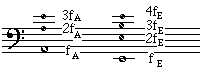 Here I use the fourth 'harmonic' on the low E string and the third 'harmonic' on the A string. The E string plays the note E2 so its fourth harmonic is E4, two octaves above. The A string plays A2, so its third harmonic is also E4, a (just) twelfth above, as shown in the diagram at right. In this video clip, I have already tuned the low E string, so here I adjust the tuning of the A string so its third 'harmonic' stops beating with the fourth 'harmonic' of the E string.
